PCA - Derivations and extensions

Background

Thanks to the development of new experimental tools for measuring neural activity, neuroscience data is rapidly increasing in its dimensionality. As a result, dimensionality reduction methods, like PCA, are becoming more and more commonplace in neuroscience research. Therefore, when I started my PhD working with these types of neural datasets, I was looking for ways to deepen my understanding of PCA so that I could better understand how / when it could be applied to my data. In this project, I document some of the excercises that helped me to strengthen my grasp on the method.

PCA is also widely used outside of neuroscience and its application include data compression, data visualization, latent variable discovery etc. Using open source tools, such as sklearn, today anyone can easily apply PCA to their data. Therefore, I hope that the following excercies might also be useful to others that are using PCA and are looking for ways to dig a little deeper into the method. A basic knowledge of PCA and linear algebra is assumed throughout the following sections.

Tools used:

numpy
scipy
sklearn
matplotlib
seaborn

Full code available at: https://github.com/crheller/PCAdemos

Outline

1. The basics
2. PCA as an eigendecomposition problem
3. PCA as a reconstruction optimization problem
4. Extensions of PCA - Sparse PCA
5. Summary

The basics

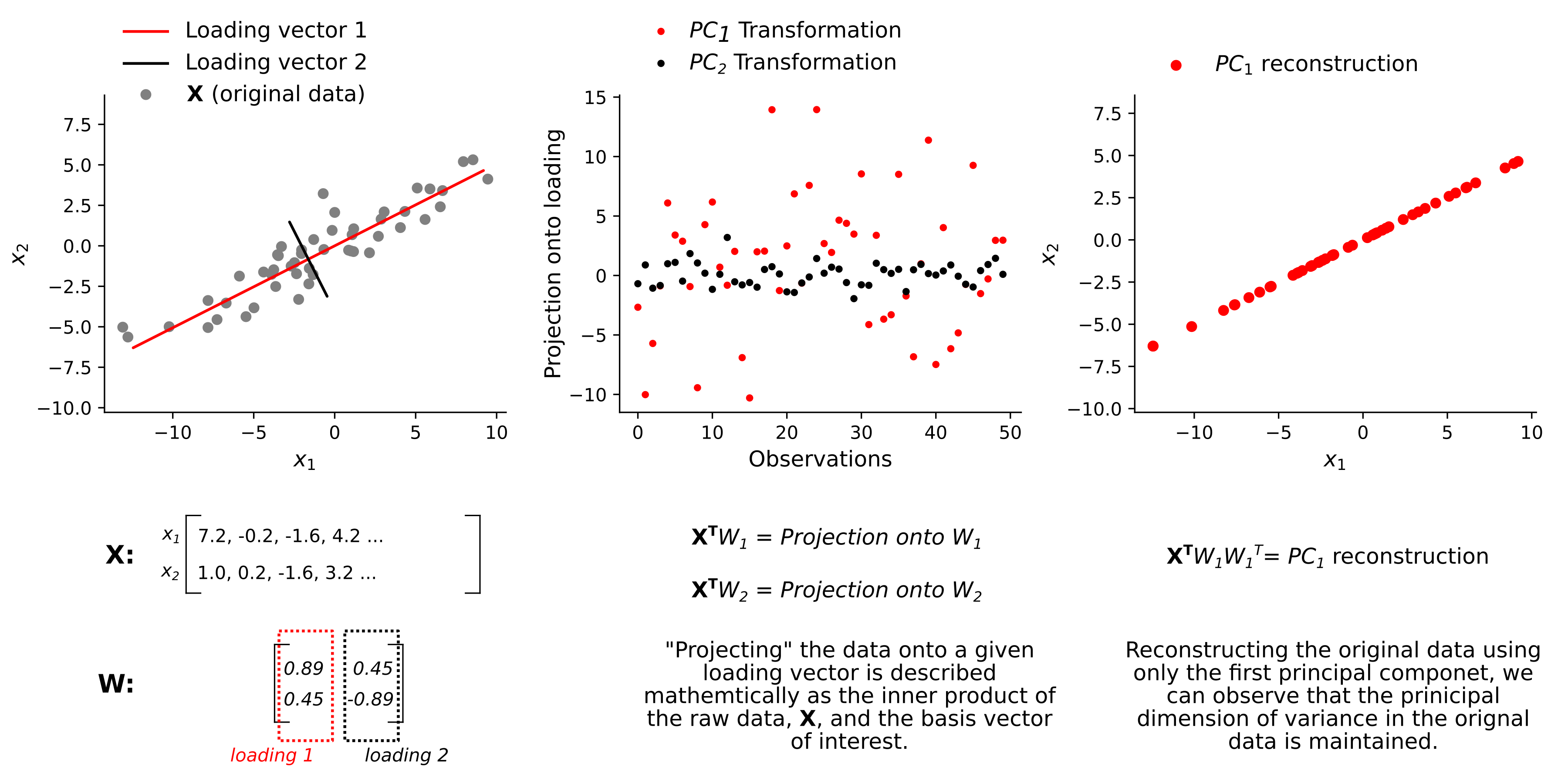
PCA is a linear dimensionality reduction method. The goal of dimensionalty reduction, in general, is to find a new represenation of the original data which maintains the data’s overall structure while also significantly reducing the number of dimensions needed to describe it. In the case of PCA, this is done by finding the ordered set of orthonormal basis vectors (called loadings) which capture the principal axes of variation in the original data. For every dataset of dimensionality \(D\), there exist \(D\) loading vectors which, together, fully capture the variance in the original data and can be thought of geometrically as describing a rotation of the original dataset. To reduce dimensionality, it is standard to discard a subset of loading vectors which capture only a small amount of variance. The number of dimensions to discard is determined by analysis of the Scree plot and can vary based on your given application. Finally, the data is transformed by projecting it onto the chosen set of loadings and using this new, low dimensional representation of the data, we can then reconstruct a “denoised”, low-rank version of the original data. The figure below gives a graphical intuition for these ideas, by applying PCA to a 2-D simulated dataset, \(\textbf{X}\).

PCA as an eigendecomposition problem

The previous section gives a general geometrical intuition for what you can achieve with PCA. However, when I started this project I wanted to learn more about how the problem is actually solved. To do this, I tried to implement PCA myself using numpy.

The most typical way PCA is solved is through eigendecomposition of the data covariance matrix, \(\Sigma\). This is the method used by most open source libraries, such as sklearn’s decomposition.PCA. Here, I step through this approach using “low level” linear algebra operations available in numpy and show that it is able to exactly reproduce the output of sklearn.

Data generation

To illustrate this approach, I again used a randomly generated 2-D synthetic data, \(X\) as above. To simplify things slightly, I generated mean-centered data (input data to PCA should always be mean-centered).

Step 1 - Compute the covariance matrix

cov = np.cov(X) # use numpy covariance function to compute covariance matrix of data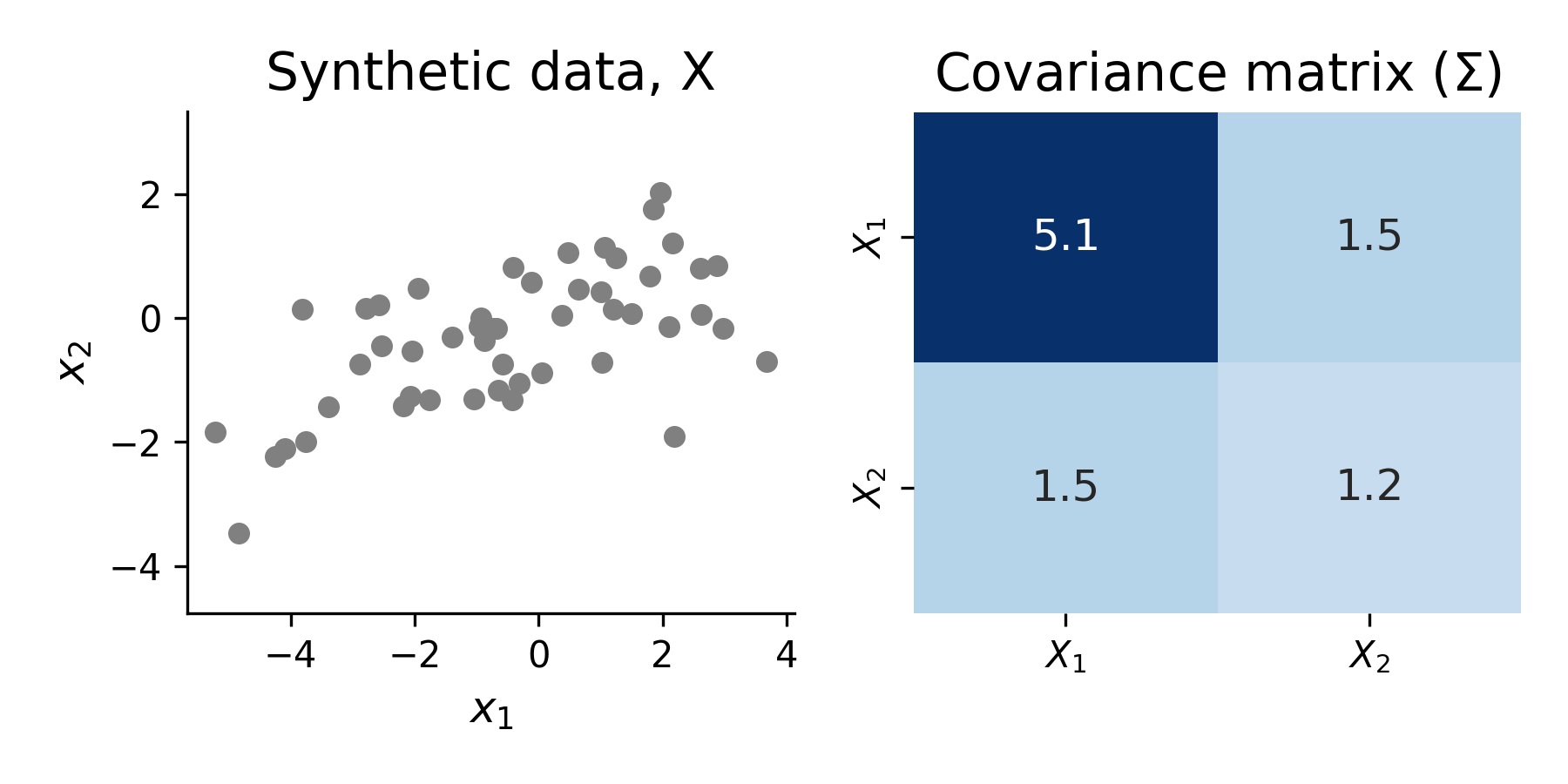

Step 2 - Perform eigendecomposition

eigenvalues, eigenvectors = np.linalg.eig(cov) 

# sort according to variance explained
sort_args = np.argsort(eigenvalues)[::-1]
eigenvectors = eigenvectors[:, sort_args]
eigenvalues = eigenvalues[sort_args]

The eigenvectors from this decomposition correspond to PC loadings and the eigenvalues are directly related to the amount of data variance along each of the corresponding eigenvectors. Thus, we can use them to calculate the % variance explained by each principal component, as shown in step 3.

Step 3 - Compute fraction variance explained by each component using eigenvalues

var_explained = eigenvalues / np.sum(eigenvalues)

Step 4 - Verify that we have reproduced sklearn results

# sklearn pca
from sklearn.decomposition import PCA
pca = PCA()
pca.fit(X.T)

Below, I show that the eigenvectors are identical to the components (loadings) returned by sklearn:

# cosine similarity -- value of 1 means the two vectors are identical. 
# Thus the inner product should return the identity matrix if the solutions match and all components are orthogonal
dp = abs.(eigenvectors.T @ pca.components_) 
print(dp)

array([[ 1.00000000e+00,  1.97596122e-16],
       [-2.21149847e-16,  1.00000000e+00]])

I also verified that the eigenvalue method for measuring % variance explained matches with sklearn:

print(f"Eigendecomposition, variance explained ratio: {var_explained}")
print(f"sklearn, variance explained ratio: {pca.explained_variance_ratio_}")

Eigendecomposition, variance explained ratio: [0.88977678 0.11022322]
sklearn, variance explained ratio: [0.88977678 0.11022322]

Finally, I used the first PC to reconstruct the original data using both methods and confirmed that, as expected, we get identical results:

e_reconstructed = X.T @ eigenvectors[:, [0]] @ eigenvectors[:, [0]].T
sk_reconstructed = X.T @ pca.components_[[0], :].T @ pca.components_[[0], :]
print(f"sum of reconstruction differences: {np.sum(e_reconstructed - sk_reconstructed)}")

sum of reconstruction differences: -1.8512968935624485e-14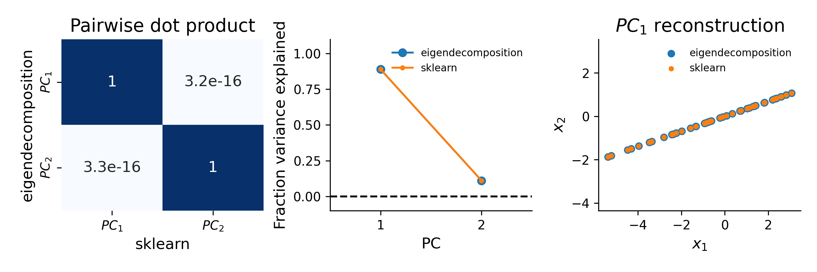

PCA as a reconstruction optimization problem

In the previous section, I showed that PCA can be formulated as an eigendecomposition problem. This approach highlighted that the covariance matrix \(\Sigma\), is a critical part of PCA. An alternative approach, however, is to formulate PCA as an optimization problem where the goal is to find the loading vector(s) that minimize the low-rank reconstruction error of the data. From an efficiency standpoint, this does not make much sense given that I just demonstrated the eigendeomposition formulation can be solved extremely efficiently. However, demonstrating that PCA can be posed as an optimization problem offers a couple of advantages. One, from an educational standpoint, it helped me to drive home the point that the objective of PCA is to find the loading vectors that can most accurately reconstruct the original data. Two, it makes it clear that we actually have flexibility to modify the objective function in order to suit our particular analysis needs. I will explore this flexibility in the following section. In this section, I demonstrate my implementation of standard PCA using scipy.

To perform PCA, we seek to minimize the objective function frob - the squared Frobenius norm of the difference between the reconstructed data and the original data:

# define objective function
def frob(pc, X):
    # reconstruct rank-1 view of X
    recon = reconstruct(pc, X)
    # compute error (sq. frob. norm of err in reconstruction)
    err = np.linalg.norm(X-recon, ord="fro") ** 2 # sq. forbenius norm
    # normalize by sq. frob norm of data, X
    err = err / (np.linalg.norm(X)**2)
    return err

Subject to the constraint that each loading vector has a magnitude of 1:

def constraint(pc):
    return np.linalg.norm(pc) - 1

Before fitting this model, I also defined a callback function in order to monitor the progress of my fitting procedure:

# define a callback function to monitor fitting progress
def callbackF(Xi):
    global Nfeval
    global loss
    global parms
    parms.append(Xi)
    ll = frob(Xi, Xfit)
    loss.append(ll)
    print(f"Nfeval: {Nfeval}, loss: {ll}")
    Nfeval += 1

Above, I have explicitly defined a constraint that ensures each loading vector has a magnitude of one. The second constraint that we must also enforce is that all loading vectors are orthogonal. To do this, I decided to perform the fitting in an iterative fashion. That is, I loop over principal components and fit one loading vector at a time. By construction, the first loading vector I find will explain the maximal amount of variance in the data. Thus, if I use this fitted loading on each iteration to deflate the target matrix \(\textbf{X}\) by subtracting the rank-1 reconstruction, I remove all variance associated with it. This means I am guaranteed that the next loading vector I find will be orthogonal to all those that were fit before it. The procedure for this is shown below:

# fit model -- iterate over components, fit, deflate, fit next PC

constraints = ({
    'type': 'eq',
    'fun': constraint
})
n_components = 2
components_ = np.zeros((n_components, X.shape[0]))
Xfit = X.copy() 
loss_optim = []
params_optim = []
for component in range(0, n_components):
    Nfeval = 1
    loss = []
    parms = []

    # initialize the PC
    x0 = np.random.normal(0, 1, X.shape[0])
    x0 = x0 / np.linalg.norm(x0)
    
    # find optimal PC using scpiy's minimize
    result = minimize(frob, x0, args=(Xfit,), callback=callbackF, method='SLSQP', constraints=constraints)
    
    # deflate X
    Xfit = Xfit - reconstruct(result.x, Xfit)

    # save resulting PC
    components_[component, :] = result.x
    
    # save all intermediate PCs and loss during the optimization procedure
    loss_optim.append(loss)
    params_optim.append(parms)

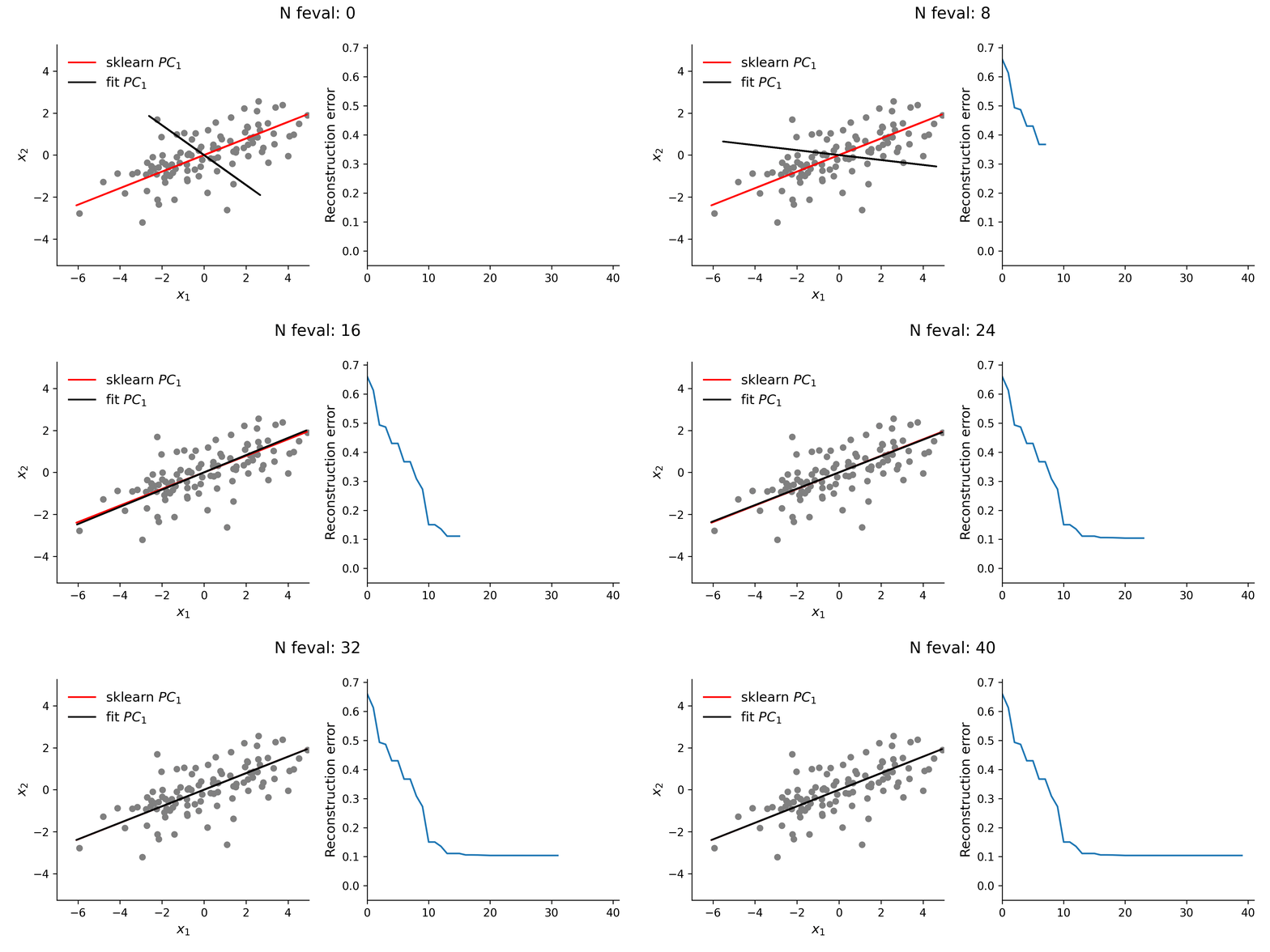
From the animation below, it is clear that the estimate of the first loading vector converges relatively quickly to the true solution given by sklearn using this procedure.

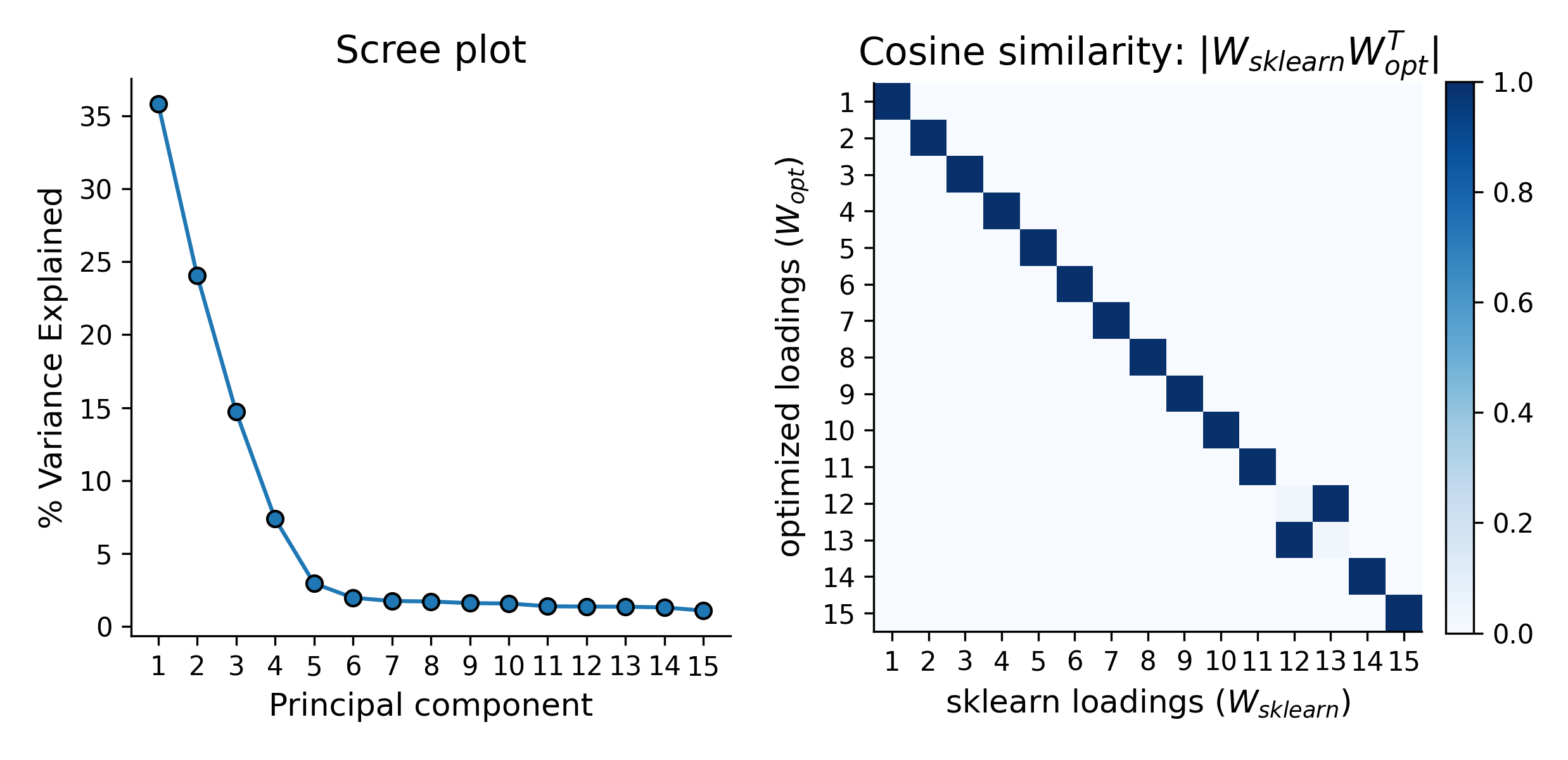
In addition to testing the above approach with simple 2-D data, I explored higher dimensional data, as well. Even with this high(er)-D data, the optimization approach is typically quite stable. However, especially for the lower variance principal components, this approach does not always guarantee finding the true solution. Thus, while illustrative, there is really no reason to use this approach for standard PCA over methods like the eigendecomposition approach.

Extensions of PCA - Sparse PCA

One advantage of thinking of PCA as an optimization problem is that one realizes how closely it parallels linear regression. This is useful because there are a variety of common extensions that exist for regression models. For example, introducing a sparsity constraint on the fitted regression coefficients (which are analogous to loading vectors, in the case of PCA). Identifying sparse loadings weights can be useful for interpretability. I was particularly interested in exploring this application because in neuroscience data the goal of population level neural data analysis is often to identify a specific subpopulation(s) of neurons that are involved in the process you are studying (e.g., encoding a sensory variable, driving behavior etc.). In my experience, this is tough to achieve with standard PCA because each loading vector is typically composed of combinations of all input neurons. Thus, sparse PC loadings have the potential to be much more biologically interpretable.

Before jumping into my implementation, I should also note that a variety of solutions have been proposed for performing Sparse PCA and packages such as sklearn often offer a version of Sparse PCA.

To implement sparse PCA “from scratch,” it is helpful to first briefly dig just a little bit into the math of the PCA objective function. In standard PCA, the goal is to minimize reconstruction error. Mathematically this can be formulated as:

Where \(\textbf{X}\) represents our original data, \(W\) represents a single loading vector, and \(\|\cdot\|_{F}^{2}\) represents the squared Frobenius norm. Thus, minimizing this function finds \(W\) such that \(\textbf{X}WW^T\) is the best possible reconstruction of \(\textbf{X}\), subject to the constraint that all \(W\) form an orthonomal basis set. This means that all vectors have a magnitude of one and are orthogonal. Mathematically, this can be expressed as \(WW^T=I\).

From this starting point, it is straightforward to introduce a sparsity penalty. One way to do this is using the L1 norm. Using the L1 norm to penalize non-sparse loading vectors, our new objective function becomes:

Where the second term, \(\sum_{i=1}^{n}\|\textbf{w}_i\|_1\) is the L1 norm and \(\lambda\) is a tunable hyperparameter that controls the level of sparsity. This new objective function is now very similar to LASSO regression. In more general terms, this adds a second “goal” that the fitter is trying to achieve – ensure that the loading weights are sparse.

To get a feel for how this might work in practice, I modified my previous implementation of the objective function to include the L1 norm as shown below:

# wrapper around frob error function that adds a L1 regularization penalty
def sparse_wrapper(pc, X, lam):
    # compute reconstruction error
    err = frob(pc, X)
    # add L1 regularization
    err = err + (np.sum(np.abs(pc)) * lam)
    return err

I then simulated datasets and fit my Sparse PCA model for a range of sparsity constraints. The effect of sparsity on the fitted loading vectors, and on the variance explained by the reconstruction, is shown in the figure below for one such simulation:

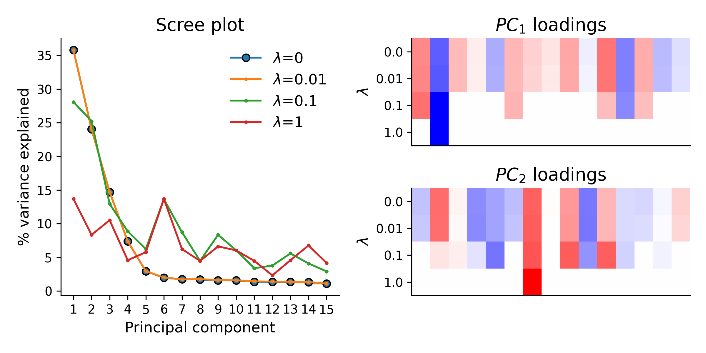
As expected, increasing \(\lambda\) leads to finding loading vectors with a more sparse set of weights. However, it also quickly reduces the amount of variance explained in the data by each of the top principal components. This is why Sparse PCA, while sometimes useful for finding interpretable loadings, is usually not a great method for other applications of PCA, such as data compression.

Summary

In this project, I briefly highlighted the basics of PCA. In addition, I demonstrated two separate methods for solving the problem from “first principles” and touched on the some of the advantages and disadvantages of each method. Finally, I showed that implementing a version of Sparse PCA is relatively straightforward, when PCA is thought of as a reconstruction optimization problem. For me, this was one of the biggest take homes - that other dimensionality reduction methods, such as Sparse PCA, Non-negative matrix factorization, Factor Analysis, etc., and their relationship to PCA, can be more easily understood when considering the underlying objective function of PCA.

All the code used in this project is saved and available on my github.