Decoding-based dimensionality reduction (dDR)

Background

One very common approach in systems neuroscience is decoding analysis. As researchers, we often ask: given neural activity alone, can we decode what the experimental condition was at any given time. The goal of this approach is typically to assign a functional label to a given neuron, group of neurons, or region of the brain. That is, if we observe that the activity of neurons in a particular region is informative about the visual environment, we can assign a “visual” label to this region. Over the years, this approach has helped researchers map out functional properties of a wide swath of brain regions.

Importantly, however, most decoding methods assume that both the first-order (mean) and second-order (variance) statistics of the data can be estimated reliably. In practice, this is not always a safe assumption, particularly today. Thanks to advances in neural recording technologies, the dimensionality of neural datasets is rapidly increasing while experimental and behavioral constraints continue to limit the amount of data (observations) that can be collected in an experiment. As a result, second-order statistics, like the activity correlations between pairs of neurons, cannot be estimated reliably in most datasets.

As a part of my PhD, I worked on developing a new, simple dimensionality reduction method which takes advantage of low-dimensional structure in neural population data to enable reliable estimation of decoding accuracy. This project was carried out under the supervision of my PhD advisor, Dr. Stephen David. Here, I will give a high level overview of the project targeted at a general, data science audience familiar with linear algebra - I will illustrate the problem, how we solved it, and demonstrate its application using example neural data. For a more in-depth, technical discussion of the method and its applications, please refer to our full manuscript.

If you are interested in trying the method with your own data, instructions for downloading the dDR package are available at: https://github.com/crheller/dDR. A demo notebook is also included in this repository which demonstrates the standard use of the method. It also contains two example extensions of the method, which are discussed in our manuscript.

What is decoding?

Decoding analysis determines how well different conditions can be discriminated on the basis of the data collected in each respective condition. To make this explanation more concrete, I will continue to focus on neuroscience data here, but keep in mind that this idea can be extended to many types of data. In a typical systems neuroscience experiment, we record brain activity from subjects while presenting sensory stimuli to study how the brain represents this information, transforms it, and uses it to guide behavior.

Let’s consider a simple experiment. Imagine that we want to know how the brain distinguishes between two different sounds - a car engine and a lawn mower. To study this, we measure the brain activity from a subject across many repeated presentations of each of these sounds. We call these presentations “trials.”

Example of simulated neural activity in response to the subject hearing the sound of a car (left) or the sound of a lawn mower (right). Red means more activity, blue means less activity.

The goal of decoding is to use the neural activity shown above to determine which dimenions of the neural activity are most informative about the sound identity. The most simple way to do this is by computing the difference in the mean activity across trials between conditions.

Example computation of decoding axis based on the mean activty in each stimulus condition. From this we can see that some neurons (e.g., neurons 8 and 9 are very informative while others (e.g., neuron 1) are less informative).

The difference in mean activity between conditions can be thought of as a “decoding axis” (\(\Delta\mu\)). Geometrically, this is the axis in the state-space of neural activity along which the mean neural activity is most different between car and lawn mower. We can visualize this by projecting the single-trial neural activities (\(X_{car}\) and \(X_{mower}\)) onto this axis:

\[r_{car} = X_{car}\Delta\mu^{T}\] \[r_{mower} = X_{mower}\Delta\mu^{T}\]

and plotting the resulting distributions for each sound:

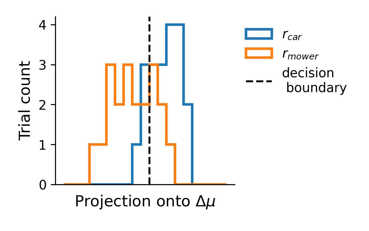
Projection of single trial activity onto the measured decoding axis.

As we can see, in this one dimensional readout of the neural activity the car and mower distributions are fairly well separated. As a final step, we can quantify the decoding performance. For example, one method for quantification would be to draw a “decision boundary,” as shown above, and determine the percentage of trials on which the sound identify was correctly identified based on the neural activity. In the following sections, however, I will use a metric called \(d'\), based on signal detection theory, which can be thought of as the z-scored difference in the response to the two stimuli:

\[d' = \| z[r_{car}] - z[r_{mower}] \|\]

Motivation for dDR

The method for decoding presented above depends only on the first-order statistics of the data - that is, only on the mean acitivty of each neuron in each condition. In some cases, however, this is not the optimal solution. Often, we can do a bit better than this if we consider not just the mean activity, but also the correlations between pairs of neurons. This is the approach taken by methods such as Linear Discriminant Analysis (LDA). To illustrate this idea, it is simpler to work with a two-dimensional dataset.

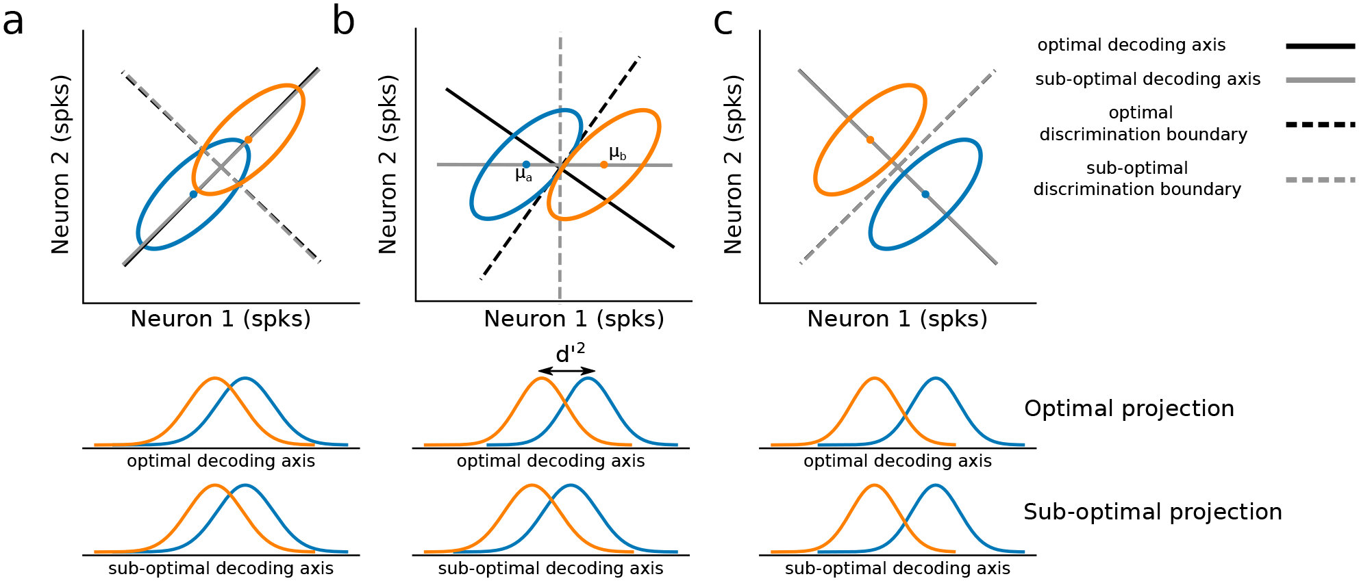
Each color represents a stimulus condition (a vs. b). Ellipses represent the variance in the responses of neuron 1 and neuron 2 across trials. The optimal decoding axis solution depends not only on the difference in the mean activity between two conditions, but also on the trial-trial covariance between pairs of neurons.

The example above illustrates that only under very special conditions (correlated activity either perfectly aligned with or perfectly orthogonal to \(\Delta\mu\)) is \(\Delta \mu\) the optimal linear decoding axis. Whenever this is not true, some benefit can be gained from factoring in correlations to the computation of the decoding axis, and a method such as LDA is preferred.

In practice, however, it is not so simple. Second-order statistics (correlations) require much more data to estimate accurately. Therefore, with limited data, estimates of neural covariance can often be innacurate. This can then lead to extreme overfitting and poor performance on heldout validation data when applying methods like LDA, as illustrated with the simulation below.

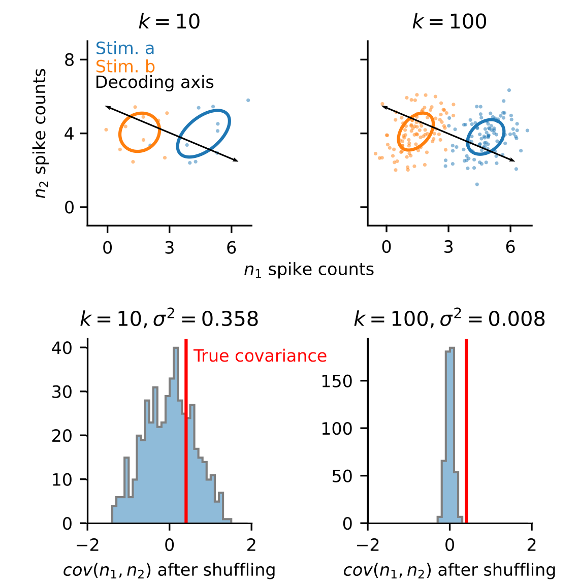
Top: Simulated response of two neurons across k=10 trials (left) or k=100 trials (right). The same underlying covariance was used in both cases. Bottom: Distribution of covariance after randomly shuffling trials between neuron 1 and neuron 2 to break all correlation. The true covariance value is well within the noise for k=10, illustrating that it cannot be estimated reliably from a sample of 10 trials. However, for k=100 trials we begin to be able to reliably measure the covariance between the pair of neurons.

In most neuroscience experiments, we operate in the regime where we have too few trials to reliably estimate covariance (i.e., reality is closest to panel a, in the figure above). Thus, if we wish to apply optimal linear decoding techniques, like LDA, we need to develop new analytical approaches to first transform our data into a format that is suitable.

dDR

dDR takes advantage of the observation that covariance patterns in neural activity are typically low-dimensional. That is, if you were to perform PCA on a typical neural dataset, you would likely find that it has a relatively small number of significant dimensions. In other words, the covariance matrix can be described using only a handful of eigenvectors (\(e\)). Unlike single pairwise covariance coefficients, these high-variance eigenvectors can be estimated reliably even from very few trials, as demonstrated in the simulation below.

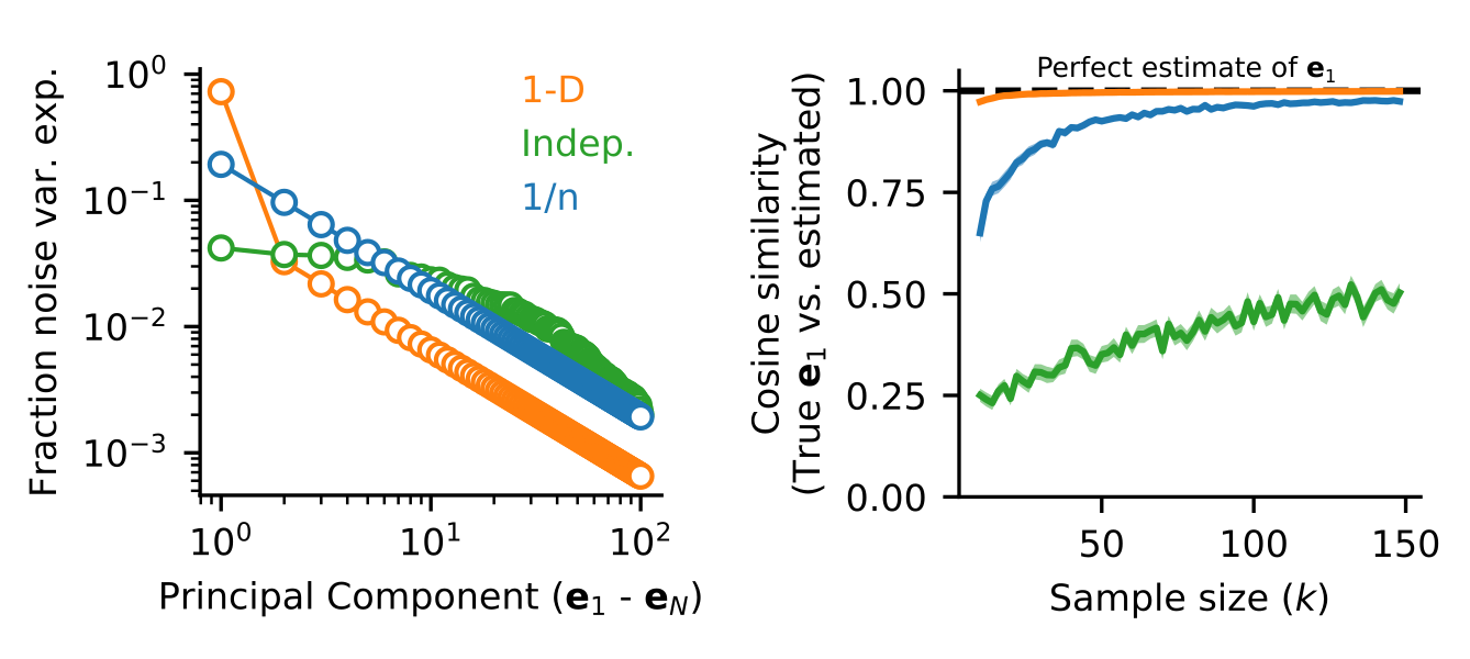
Left: Scree plot for 3 simulated datasets - One with low dimensionality (1-D), one with covariance that decays according to power law (1/n), and one where the variance of each neuron is independent (indep.). Right: Quality of the first principal component estimate as a function of number of trials.

Thus, the first principal component of trial-trial covariance and the respective mean of neural activity under each condition define a unique hyperplane in the neural activity state space which can 1. Be estimated robustly and 2. Captures the two key features of population activity required for optimal linear decoding analysis. We call the projection into this space dDR. The full procedure is sketched out graphically below:

Schematic of the stepwise procedure for projecting high-dimensional data into the dDR space.

Once projected into the dDR space, we can perform our optimal linear decoding analysis of choice without as much concern about overfitting to noisy estimates of pairwise covariance. Thus, dDR can be viewed as a sort of regularization to be performed prior to estimating decoding accuracy. In the next two sections, we briefly highlight dDR’s application to simulated and real data.

Application to neural data

The sensitivity of decoding methods to overfitting is a known problem in neural data analysis. This is commonly dealt with by either using the \(\Delta \mu\) decoding approach discussed in section 1 or to reduce the dimensionality of the data using principal component analysis. While each of these approaches are valid, they often result in finding non-optimal solutions. To illustrate this, we applied all three methods (\(\Delta\mu\), PCA, and dDR) to the same dataset and compared their cross-validated decoding performance as a function of number of trials.

Neural activity was recorded from 52 neurons in auditory cortex while subjects listened to 50 repeats of 4 different auditory stimuli. Decoding performance for stimulus 1 vs. stimulus 2 (top) and stimulus 3 vs. stimulus 4 (bottom) is shown here. Left panels show the projection of 52-dimensional data into the 2-dimensional dDR space. Decoding performance (right) was measured as a function of trial count and was normalized to dDR performance. Stimulus repetitions were subsampled to show how decoding performance changes as a function of the number of trials.

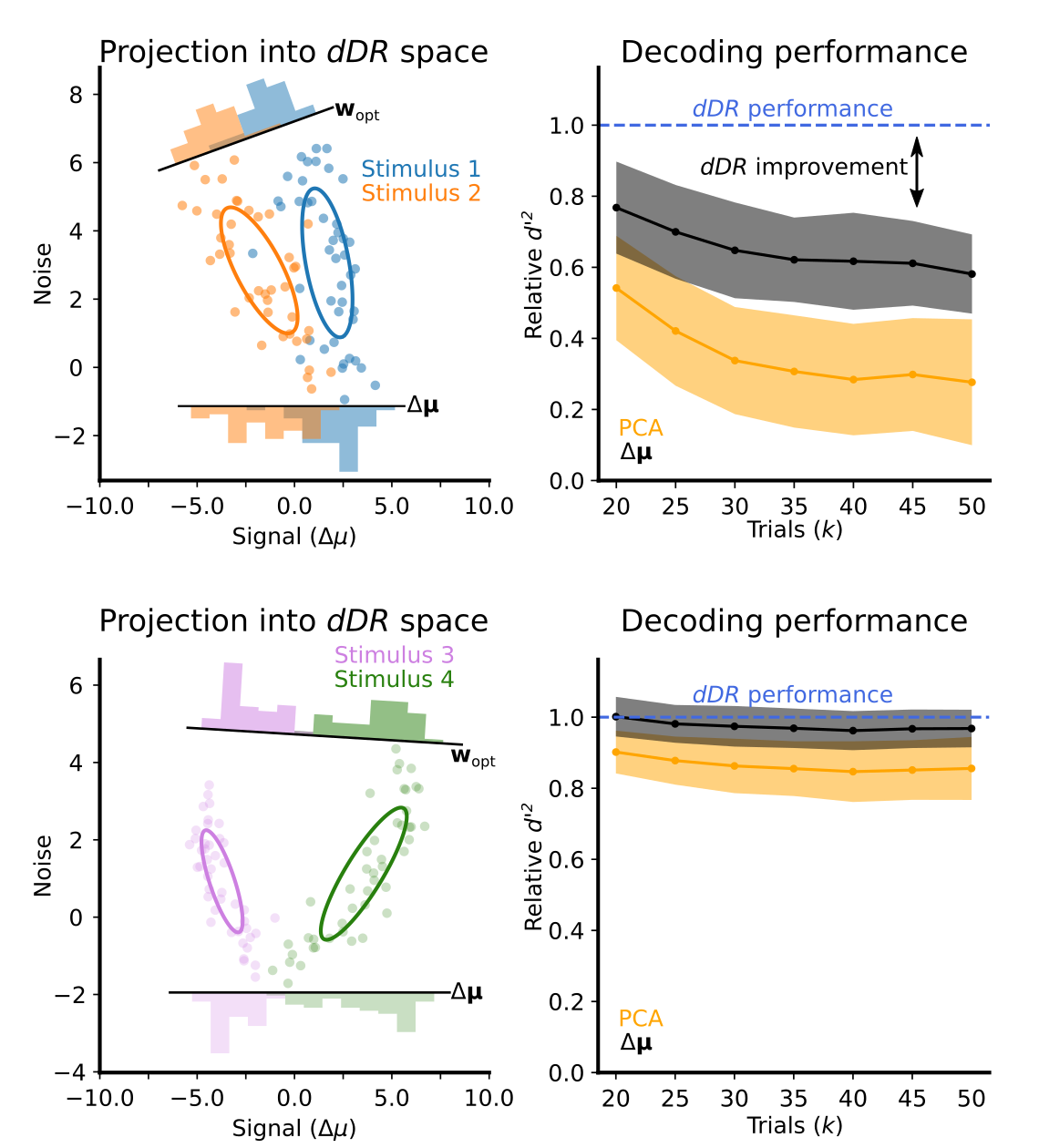
In all cases, we found that dDR performed as well as, or better than, both \(\Delta \mu\) and PCA approaches. We found that dDR was particulary beneficial in cases where 1. The two stimuli evoked similar mean activity in the neurons and 2. When the principal axis of covariance was not perfectly aligned with, or orthogonal to, the \(\Delta \mu\) axis, as discussed in section 2.